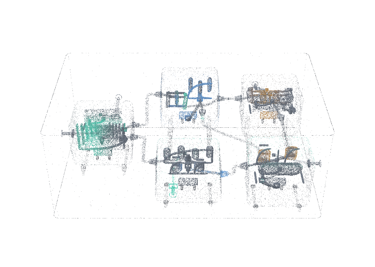
Metahive Builder

Every configuration has consequences.

Metahive Builder is a 3D planning tool for compute-site planners, so that they see whether space, power, cooling or memory runs out first, before buying hardware.

  • Infrastructure
  • Data center planners
  • 3D site simulation
  • Power & heat modeling
Containment, physical limits and workload calculation. An illustrative design calculation under explicit equipment and workload assumptions.
Loading model
Technical descriptionsInteractive model unavailable. The static illustration and descriptions remain available.
Hierarchical configuration
Place devices within racks, rooms, buildings and plot with sourced assumptions.
Technical data

Inputs

Tagged equipment and site assumptions.

One explicit revised equipment assumption; preserve the original baseline.

Transformation

Place devices within racks, rooms, buildings and plot with sourced assumptions.

Retained state and outputs

Fit, aisle, mass, floor load and site assumptions.

Original configuration and changed input remain identifiable.

Constraints

Physical fit and site assumptions retain their source and units.

Electrical and thermal propagation
Keep distinct power bases and propagate losses, heat and cooling demand.
Technical data

Inputs

Equipment/power assumptions with containment context.

Transformation

Keep distinct power bases and propagate losses, heat and cooling demand.

Retained state and outputs

Nameplate, provisioned peak and utilization basis.

IT heat, conversion losses and facility demand.

Constraints

Nameplate, provisioned peak and utilization are different power bases.

Inference workload model
Derive memory and throughput bounds from the workload and selected equipment.
Technical data

Inputs

Selected capacity and placement.

Model shape, precision, context and concurrency.

Transformation

Derive memory and throughput bounds from the workload and selected equipment.

Retained state and outputs

Weights, workspace, KV memory, precision and concurrency.

Compute/memory bounds and selected utilization assumptions.

Constraints

An infeasible memory requirement prevents an operating-energy result for that configuration.

Time and energy scenario
Balance load, supply, storage and grid under the selected time basis.
Technical data

Inputs

Calculated facility load under the selected power basis.

Duration/weather/supply/storage assumptions.

Transformation

Balance load, supply, storage and grid under the selected time basis.

Retained state and outputs

Load, generation, exchange, shortfall and storage state.

Base/low/high inputs and their source quality.

Constraints

Time-based supply and storage remain balanced, including shortfall.

Constraint and alternative comparison
Join physical and workload results and expose the binding constraint.
Technical data

Inputs

Electrical and thermal feasibility.

Memory feasibility and workload bounds.

Calculation with its time basis, not an observed operating result.

Transformation

Join physical and workload results and expose the binding constraint.

Retained state and outputs

Feasible, failed and unresolved results.

Units, method, input lineage and comparison basis.

Constraints

Calculated feasibility is an illustrative evaluation, not commissioned hardware performance.

An illustrative design calculation under explicit equipment and workload assumptions.

Additional mechanisms are described in the technical reference.

The site hierarchy feeds electrical, thermal and workload calculations. Compare the resulting limits with the time-based energy scenario to identify the binding constraint.

Move one rack. See what else changes.

Discuss a site scenario

What the research says

Site energy is now reported, and soon rated.

Regulators now ask for a site’s energy performance and plan to rate it, while the industry’s headline efficiency figure has stood still. A planner has to defend those numbers before the hardware arrives. Builder computes them from the layout and shows the assumptions behind each one.

A placement changes more than the floor plan.

A planned rack move can change equipment fit, electrical loading and cooling across the room. The planner needs to see those consequences while comparing the layout and the workload it is meant to support.

Use Builder while evaluating a fitout, a different device mix or a changed inference workload. Start with the physical hierarchy and sourced assumptions, then inspect which constraints change as the configuration changes. Its engineering and financial scenarios retain their input quality and assumptions.

Device → rack

Check equipment fit, weight, clearances and electrical demand.

Rack → room

Follow cooling, airflow, floor loading and containment across neighboring equipment.

Room → site

Connect the building and plot to power paths, land use and operating assumptions.

Two limits meet in the same configuration.

A compute design must support both its physical demand and its intended workload.

The energy model

Nameplate rating, provisioning peak, component load and utilization-dependent energy remain separate. PSU losses, redundancy and cooling add their own requirements.

The inference model

Weights, KV cache, tensor-parallel placement, batch and concurrency determine memory needs. Compute and memory rooflines bound the workload a configuration can support.

The operating day

Hourly scenarios connect generation, storage, grid caps and cooling. A favorable design-point ratio cannot stand in for an annual energy quantity.

What happens if we move one rack?

A site planner changes one thing; Builder recomputes power, cooling and inference under the same assumptions. Illustrative.

  1. 1 of 4A site planner moves one rack to the end of the row to free floor space. Nothing else is changed by hand.Decision: Where the rack goes.
  2. 2 of 4The rack now draws from a different power feed, and that feed’s load and headroom are recomputed.
  3. 3 of 4Cooling follows: the rack’s heat now lands on another part of the cooling path, and the cooling load is recomputed.
  4. 4 of 4Inference capacity is recomputed under the same assumptions, and the planner sees which limit binds first.Decision: Keep the move or try another position.
Select any part of the drawingScroll to step · Esc to skipFig. 1
  1. 1 of 4The planner saves the current layout as design A and copies it as design B.
  2. 2 of 4In design B, two racks take a denser device mix. The workload and the outdoor-temperature scenario stay fixed for both.
  3. 3 of 4Builder reruns power, cooling and memory for both designs from the same shared assumptions.
  4. 4 of 4The planner compares which constraint binds in each design and opens the calculation behind the difference.Decision: Which design to take forward.
Select any part of the drawingScroll to step · Esc to skipFig. 1
  1. 1 of 4The site’s grid connection has a cap. The planner enters it as a limit on the plan.
  2. 2 of 4An hourly scenario runs generation, battery storage and grid exchange against the site’s load across the year.
  3. 3 of 4In the hottest hours the cooling load rises, the cap is reached, and Builder records the unmet load hour by hour.
  4. 4 of 4The planner weighs the options: add storage, lower the planned load, or accept a smaller workload.Decision: Add storage, lower the load or shrink the workload.
Select any part of the drawingScroll to step · Esc to skipFig. 1

Inside the mechanism. One changed workload. A traceable design decision.

A synthetic inference scenario follows concurrency into KV memory, a capacity choice and a one-hour energy scenario. Every numerical input is an assumption; none is a hardware benchmark.

The first workload fits the assumed memory domain.

Sixteen sequences require 40 GiB. The selected 48 GiB option fits this memory calculation.

Open the memory calculation.

All numerical inputs below are synthetic assumptions. This is one memory domain, not a measured rack or device.

Model layers
32
KV heads
8
Head dimension
128
Bytes per element
2
Context tokens
8192
Concurrent sequences
16

KV bytes = 2 × layers × KV heads × head dimension × bytes per element × context × concurrency

KV GiB = KV bytes ÷ 1,073,741,824 (2³⁰).

KV-cache method reference. Full uniform KV allocation; no paging, prefix sharing, quantization or sliding-window reduction is assumed.

20 GiB weights + 4 GiB workspace + 16 GiB KV = 40 GiB required

48 GiB assumed usable capacity.

8 GiB remaining under these assumptions.

Device design power
0.55 kW, assumed for the selected option
Other IT load
0.45 kW, assumed
IT design load
0.55 kW device + 0.45 kW other IT = 1 kW
IT feed limit
1.3 kW: within the declared budget
Heat-removal limit
1.4 kW: within the declared budget
Facility scenario
1 kW × 1.2 assumed facility ratio = 1.2 kW
One constant-load hour
1.2 kWh under the constant-load assumption

Concurrency changes memory demand. Power changes only when a separately assumed device option is selected. Memory fit is necessary; throughput, physical installation and site acceptance need their own evidence.

The same option no longer fits.

Thirty-two sequences need 56 GiB against 48 GiB. The workload remains unresolved; no successful operating-energy result is assigned.

Open the memory calculation.

All numerical inputs below are synthetic assumptions. This is one memory domain, not a measured rack or device.

Model layers
32
KV heads
8
Head dimension
128
Bytes per element
2
Context tokens
8192
Concurrent sequences
32

KV bytes = 2 × layers × KV heads × head dimension × bytes per element × context × concurrency

KV GiB = KV bytes ÷ 1,073,741,824 (2³⁰).

KV-cache method reference. Full uniform KV allocation; no paging, prefix sharing, quantization or sliding-window reduction is assumed.

20 GiB weights + 4 GiB workspace + 32 GiB KV = 56 GiB required

48 GiB assumed usable capacity.

8 GiB beyond capacity. This workload remains unresolved.

Device design power
0.55 kW, assumed for the selected option
Other IT load
0.45 kW, assumed
IT design load
0.55 kW device + 0.45 kW other IT = 1 kW
IT feed limit
1.3 kW: within the declared budget
Heat-removal limit
1.4 kW: within the declared budget
Facility scenario
Unresolved: no successful operating-energy result is assigned.
One constant-load hour
Unresolved

Concurrency changes memory demand. Power changes only when a separately assumed device option is selected. Memory fit is necessary; throughput, physical installation and site acceptance need their own evidence.

A separate equipment assumption changes the scenario.

The assumed 80 GiB option fits the memory requirement. Its independently assumed design power is higher; the feed, cooling and facility scenario are checked again.

Open the memory calculation.

All numerical inputs below are synthetic assumptions. This is one memory domain, not a measured rack or device.

Model layers
32
KV heads
8
Head dimension
128
Bytes per element
2
Context tokens
8192
Concurrent sequences
32

KV bytes = 2 × layers × KV heads × head dimension × bytes per element × context × concurrency

KV GiB = KV bytes ÷ 1,073,741,824 (2³⁰).

KV-cache method reference. Full uniform KV allocation; no paging, prefix sharing, quantization or sliding-window reduction is assumed.

20 GiB weights + 4 GiB workspace + 32 GiB KV = 56 GiB required

80 GiB assumed usable capacity.

24 GiB remaining under these assumptions.

Device design power
0.8 kW, assumed for the selected option
Other IT load
0.45 kW, assumed
IT design load
0.8 kW device + 0.45 kW other IT = 1.25 kW
IT feed limit
1.3 kW: within the declared budget
Heat-removal limit
1.4 kW: within the declared budget
Facility scenario
1.25 kW × 1.2 assumed facility ratio = 1.5 kW
One constant-load hour
1.5 kWh under the constant-load assumption

Concurrency changes memory demand. Power changes only when a separately assumed device option is selected. Memory fit is necessary; throughput, physical installation and site acceptance need their own evidence.

Where it changes the work.

Illustrative situations, connected to the mechanisms that make them possible.

Design the datacenter before the fitout

Datacenter designers

Racks must fit the room while power, cooling and floor constraints remain credible.

How it works
Nested geometry checks connect equipment placement to its building and plot.
What changes
A layout can reveal a physical conflict before it is mistaken for an available capacity.

See what changes with another model

AI infrastructure teams

A model’s precision and context length change memory and inference requirements.

How it works
Weights, KV cache, parallelism and rooflines propagate the workload into the configuration.
What changes
The team can compare a workload envelope instead of buying from accelerator count alone.

Compare an energy and investment scenario

Operators and investment planners

A denser design changes electrical demand, heat, annual energy and cost assumptions.

How it works
Power and thermal propagation share a scenario basis with annual weather, supply and storage.
What changes
The decision retains units, input quality and sensitivity instead of presenting one unexplained ROI figure.

Compare the change under the same assumptions.

Consider replacing a rack configuration while keeping the workload and ambient scenario fixed.

  1. Change one input

    Update equipment or workload and retain the comparison basis.

  2. Find the binding constraint

    Inspect the electrical, thermal or memory limit that prevents the intended operation.

  3. Open the calculation

    A result keeps its units, method, input lineage and source quality. Assumptions and defaults remain available for scrutiny.

Questions about Metahive Builder.

Are the inference figures measured benchmarks?

Builder produces calculated bounds and scenarios from its declared models and inputs. Hardware benchmarking is a separate activity.

Can Builder guarantee project returns?

It informs technical feasibility and operating assumptions. Financial feasibility also requires independently checked costs, demand, financing and contractual terms.

Metahive Builder in the stack.

Built on

Infrastructure program

A planning tool within the wider compute and site direction.

Connected system

Deployment constraints

Custody and model access can become design requirements.

Technical reference6 mechanisms · 3 further sections

The mechanisms underneath.

The technical choices that give Metahive Builder its particular behavior.

Device → rack → room → building → plot
Nested placement gives every device a physical context. Containment, equipment fit, aisle clearance, floor load and site constraints can be checked as the configuration changes.
Power propagates into heat
Nameplate, provisioned peak and utilization are different power bases. PSU losses, IT heat, cooling and facility demand are propagated through the same scenario.
Inference has a memory and throughput bound
Model weights, KV cache, precision, tensor parallelism and compute/memory rooflines determine the workload envelope. Installed accelerator count alone cannot describe useful capacity.
A year can change the design
Weather, energy supply, storage and cooling assumptions shape annual scenarios. Compare design choices on the same input basis and expose the assumptions that dominate the result.
Every result has units and provenance
Inputs retain their source, quality grade and method. Rated values, assumptions and measured observations remain distinguishable inside a visually precise design.
Engineering and investment stay connected
A physical configuration can inform capital, operating-cost and sensitivity scenarios. Financial planning retains its own assumptions; a detailed model does not turn an estimate into a promised return.

A placement changes more than the floor plan.

Metahive Builder couples a 3D site hierarchy with electrical, thermal, energy and inference scenarios. A configuration change reveals its constraints, and each calculation retains its units, method and input lineage.

Device → rack. Check equipment fit, weight, clearances and electrical demand.

Rack → room. Follow cooling, airflow, floor loading and containment across neighboring equipment.

Room → site. Connect the building and plot to power paths, land use and operating assumptions.

Two limits meet in the same configuration.

The energy model. Nameplate rating, provisioning peak, component load and utilization-dependent energy remain separate. PSU losses, redundancy and cooling add their own requirements.

The inference model. Weights, KV cache, tensor-parallel placement, batch and concurrency determine memory needs. Compute and memory rooflines bound the workload a configuration can support.

The operating day. Hourly scenarios connect generation, storage, grid caps and cooling. A favorable design-point ratio cannot stand in for an annual energy quantity.

Compare the change under the same assumptions.

Change one input. Update equipment or workload and retain the comparison basis.

Find the binding constraint. Inspect the electrical, thermal or memory limit that prevents the intended operation.

Open the calculation. A result keeps its units, method, input lineage and source quality. Assumptions and defaults remain available for scrutiny.

System story

From a device to a useful compute site

A proposed compute-site scenario showing the relationship between equipment, energy and inference.

Follow the story

Which limit would your next site hit first?

Discuss a site scenario